A few months back I dove into a book on making sense of complex data with simple models as a part of my research (High-Dimensional Data Analysis with Low-Dimensional Models, by Wright and Ma). I learned about and implemented a fun demo of Principal Component Pursuit (PCP). My advisor loved it! We played with feeding the algorithm different kinds of simulated data, and wondered about how we might apply such an idea to better understand 3D tomograms.

Recently my advisor was out of town. He’s currently introducing a new class on scientific computing (Computational Physics, PHSCS 530) here at BYU. I was surprised when he asked me to fill in for him, teaching about my Principal Component Pursuit project!

In preparation, I cleaned up my code a little, made a new demonstration, and prepared my lecture. It went really well, and taught me so much.

Here I’ve essentially written out what I taught the class, minus a few side tangents about machine learning and dimensionality reduction from questions that students asked.

Read on to learn about it!

A lesson on Principal Component Pursuit #

Presentation Slides (Google Slides)

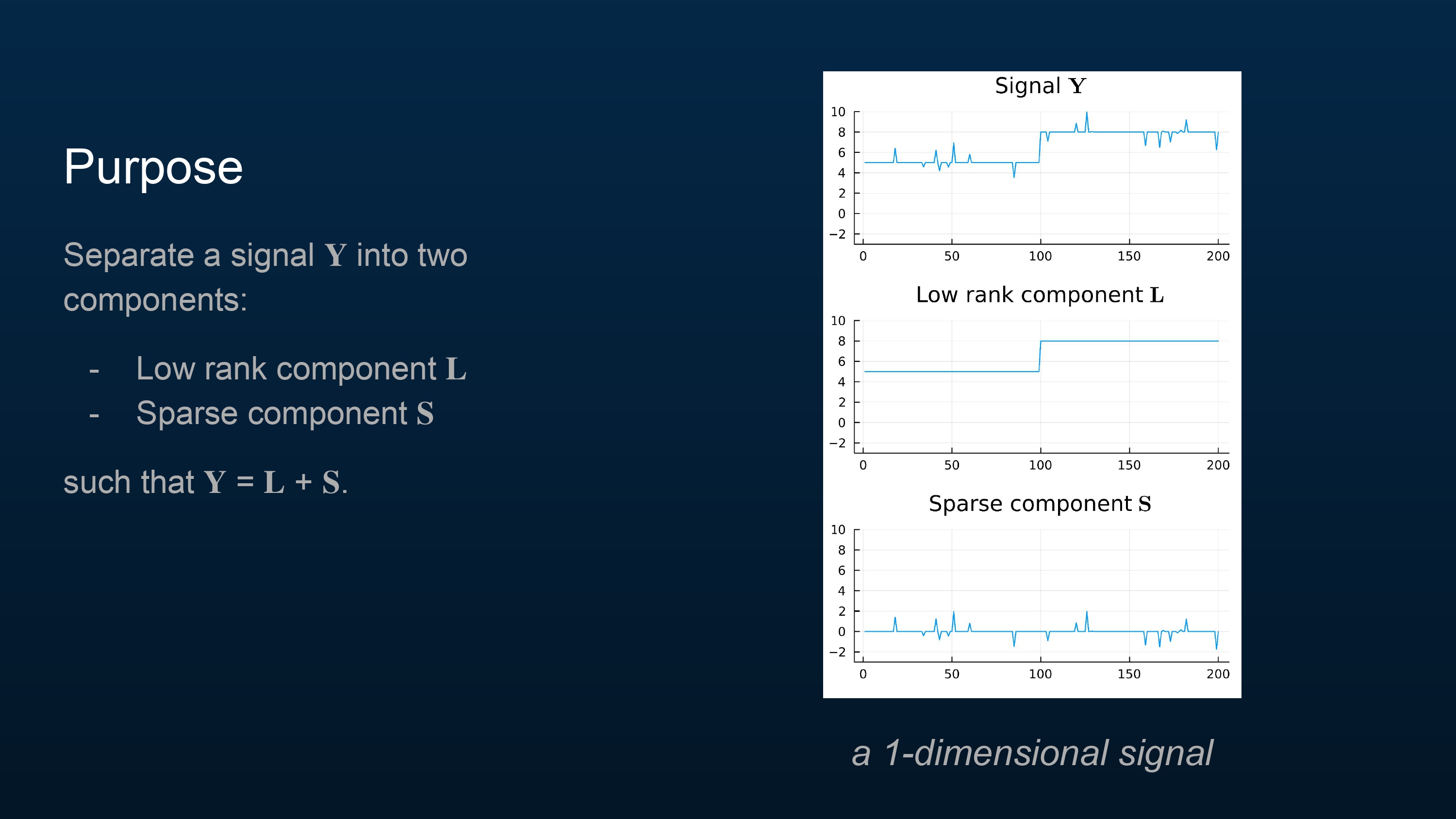
A signal $\bf{Y}$ can often be broken up into two parts—a part that stays mostly the same over time ($\bf{L}$), and part that is usually zero ($\bf{S}$).

To formalize what this means, we say that $\bf{L}$ should be low rank, and $\bf{S}$ should be sparse.

The plot in the slide provides some intuition for what a sparse signal is. You can see that $\bf{S}$ is usually zero (it is sparse), and the original signal $\bf{Y}$ is the sum of the two components $\bf{L}$ and $\bf{S}$.

The plot can’t depict a low-rank signal well since this signal $\bf{Y}$ is only one-dimensional, but a low-rank signal in this context may be understood as a signal that stays mostly the same, most of the time. In a moment we will look at a higher dimensional signal and talk more about this.

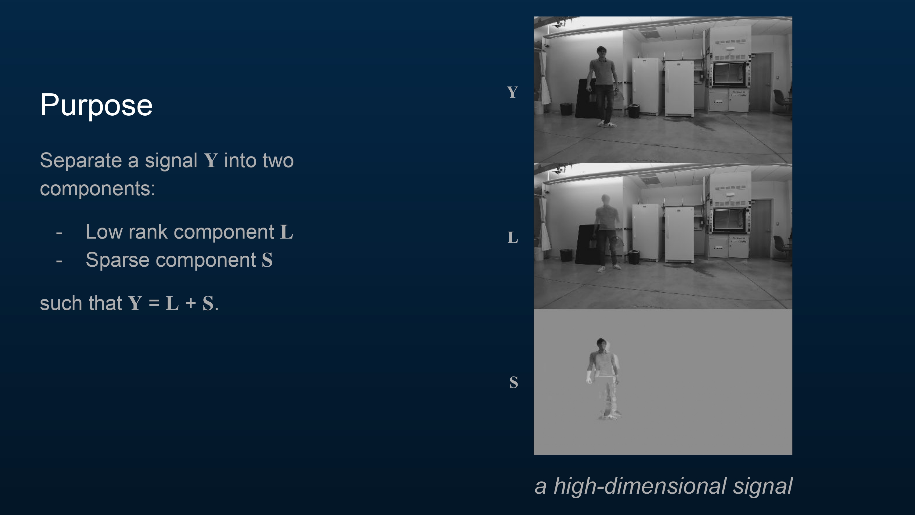
A video is a high dimensional signal! Just as the previous plot showed a signal decomposed into a low-rank and a sparse component, here is a short video of me in my lab decomposed in a similar way, to motivate what I’m about to share with you.

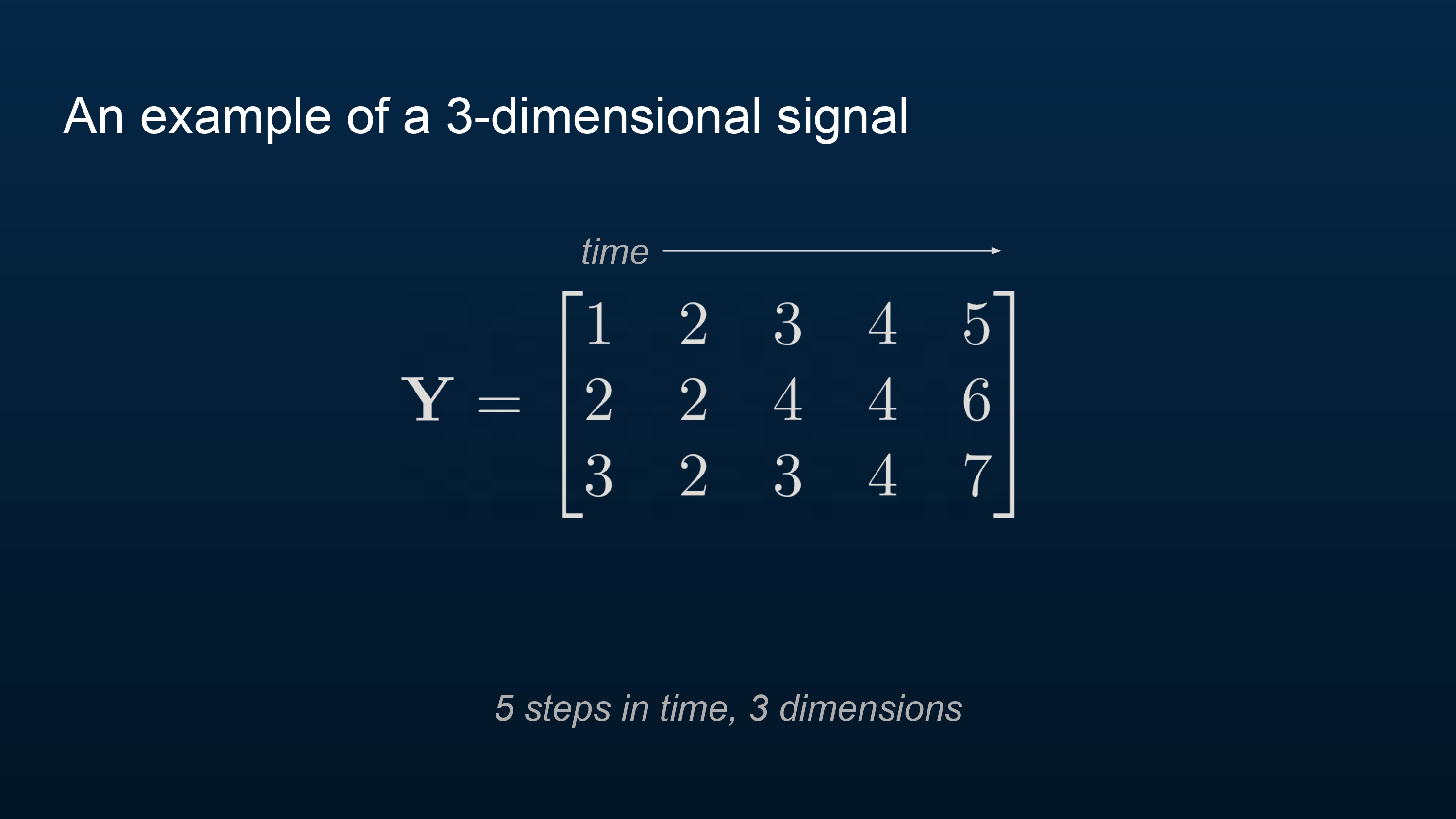
Here is a three-dimensional signal. Each column represents the signal at a point in time.

The rank of a matrix is the number of linearly independent columns (or rows) in the matrix. Here $\bf{Y}$ is full-rank, meaning that the rank is as high as possible for a matrix of this size ($\text{rank}(\bold{Y}) = 3$). (Given an $m \times n$ matrix, the highest the rank can be is the smallest dimension, either the number of rows $m$ or the number of columns $n$.)

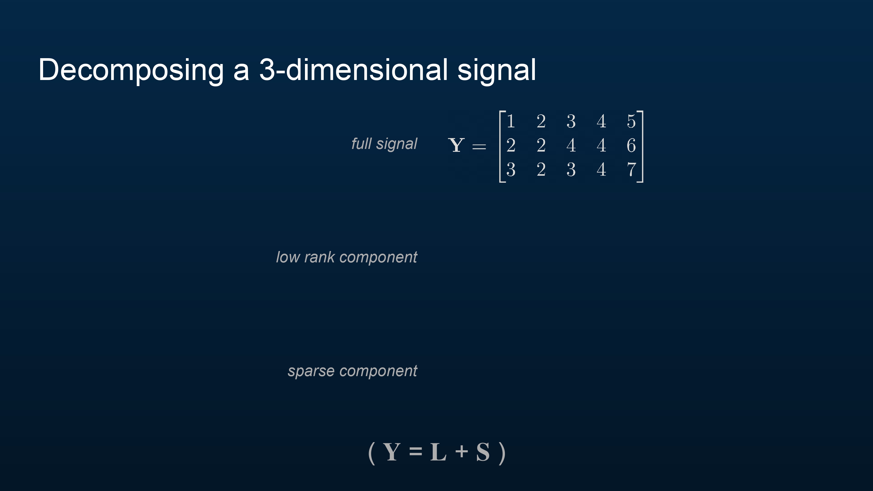
Now we will decompose $\bold{Y}$ into a low-rank and a sparse component such that $\bold{Y} = \bold{L} + \bold{S}$. What do you think this will look like?

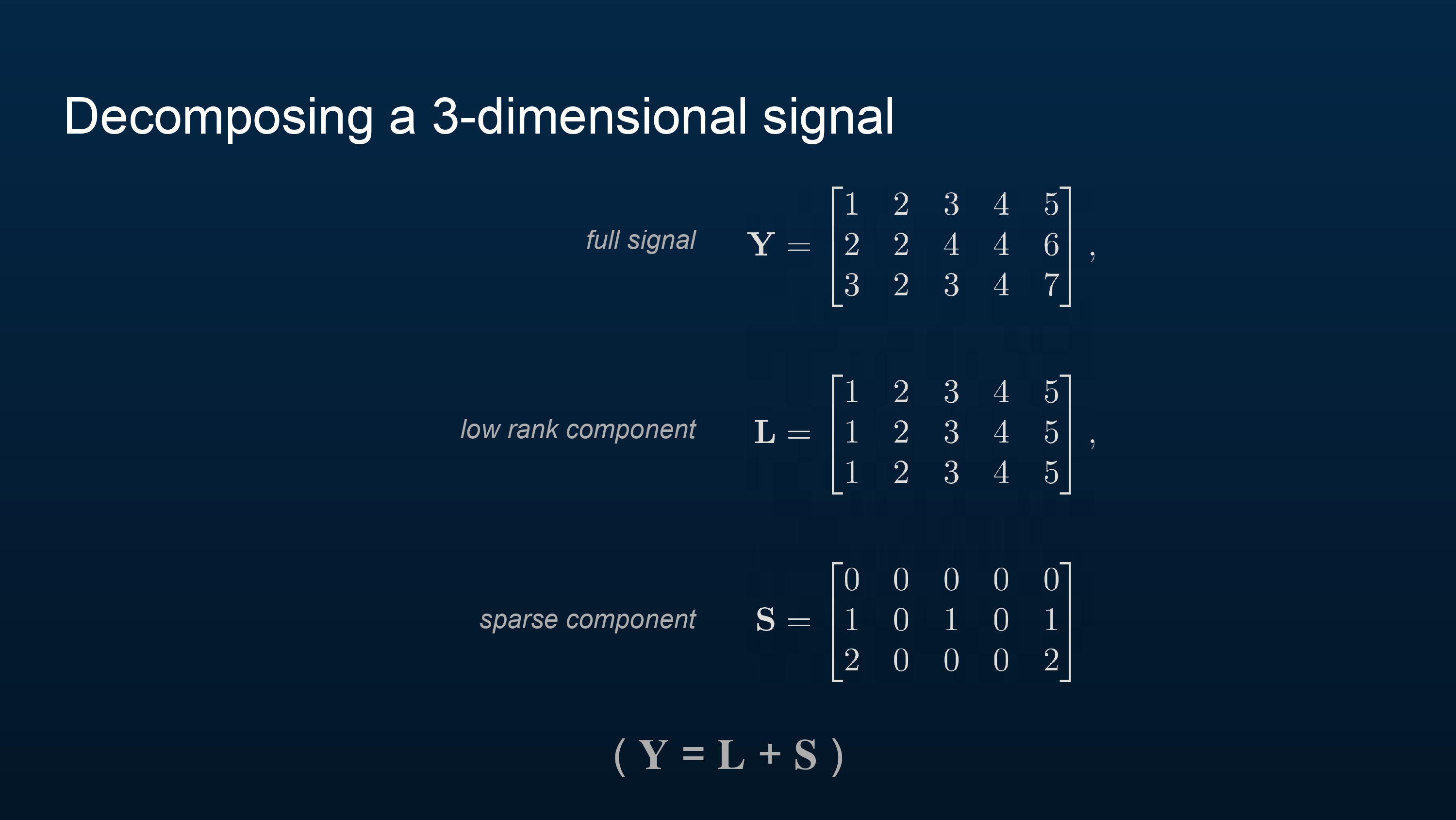
Here is one good decomposition. The rank of $\bold{L}$ is as low as possible—just 1! Meanwhile, $\bold{S}$ is somewhat sparse, with only 5 nonzero elements. And, as desired, $\bold{Y} = \bold{L} + \bold{S}$.

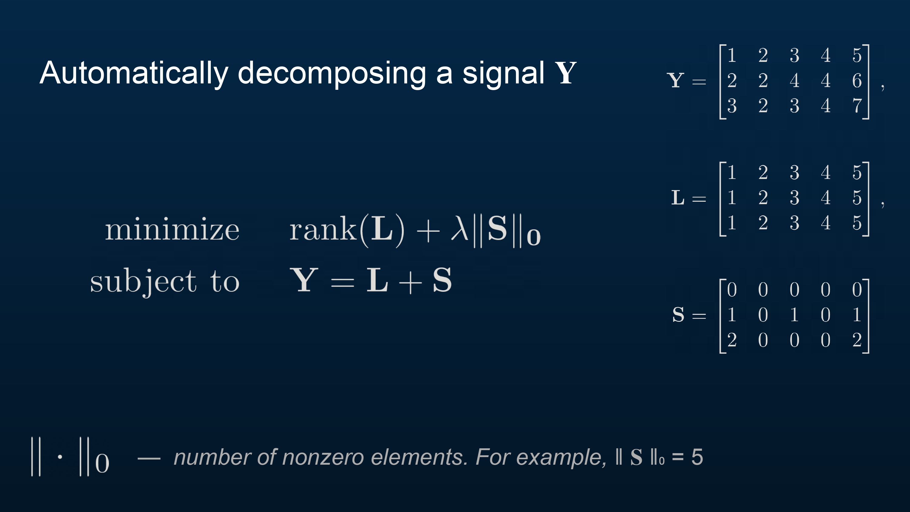
How might we formalize and automate such a decomposition? We want the rank of $\bold{L}$ and the number of non-zero elements of $\bold{S}$ to both be low. So let’s minimize that, with a parameter $\lambda > 0$ to control the relative importance of each.

And to make sure it’s a true decomposition of $\bold{Y}$, we add the condition that $\bold{Y} = \bold{L} + \bold{S}$.

This problem perfectly describes our goal mathematically, but it is hard to program a routine that does this automatically. It isn’t a convex problem, so we cannot expect it to have unique optimizers (in other words, we cannot expect there to be a unique $\bold{L}$ and $\bold{S}$ that minimize $\text{rank}(\bold{L}) + \lambda \Vert \bold{S} \Vert_0$). Solving this problem automatically would be very hard.

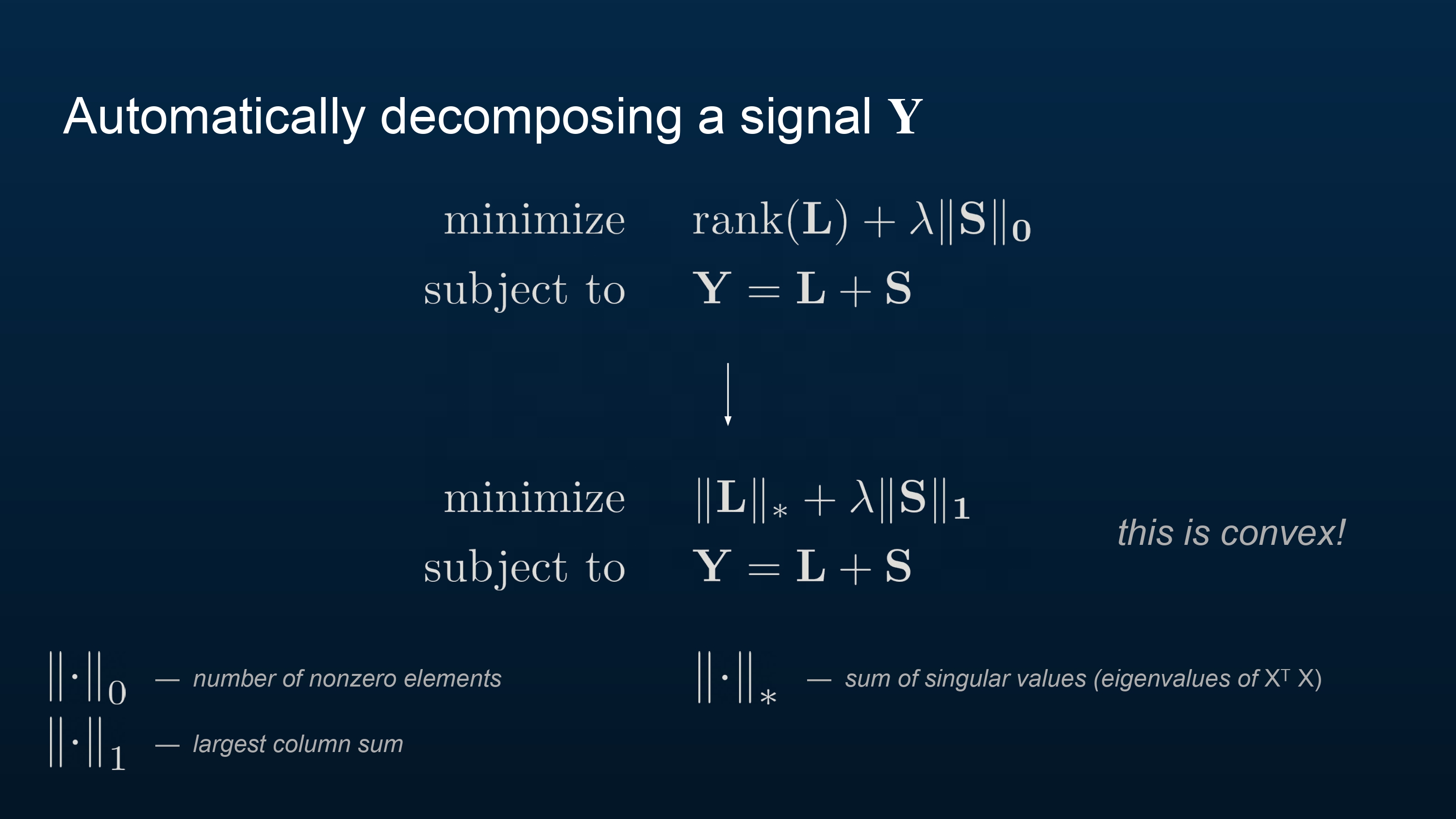
So we set up a similar problem that is easy to solve. We want to make the problem convex, a mathematical condition that implies that any local minimum of the problem is also a global minimum—generally, this means that there is a unique optimizer for the problem, which will make it easy to solve.

We replace $\text{rank}(\bold{L})$ with the nuclear norm of $\bold{L}$, denoted $\Vert \bold{L} \Vert_*$. This represents the sum of the singular values of $\bold{L}$, which are closely tied to its eigenvalues. In particular, if $\bold{L}$ has a low rank, then most of $\bold{L}$’s singular values are zero. (Specifically, $\text{rank}(\bold{L}) = \Vert \boldsymbol{\sigma}(\bold{L}) \Vert_0$ where $\boldsymbol{\sigma}(\bold{L})$ yields the singular values of $\bold{L}$). This norm is convex.

We replace $\Vert \bold{S} \Vert_0$ with the largest column sum (taking the absolute value of each element) of $\bold{S}$, denoted $\Vert \bold{S} \Vert_1$. If most of the elements of $\bold{S}$ are 0, then we may safely assume that the largest column sum of $\bold{S}$ will be small, barring the possibility that the non-zero elements of $\bold{S}$ are huge in magnitude. This norm is also convex.

The new problem we have constructed is convex, and thus, any $\bold{L}$ and $\bold{S}$ that minimize the problem locally also minimize it globally! This makes our search much easier. We call this new problem Principal Component Pursuit.

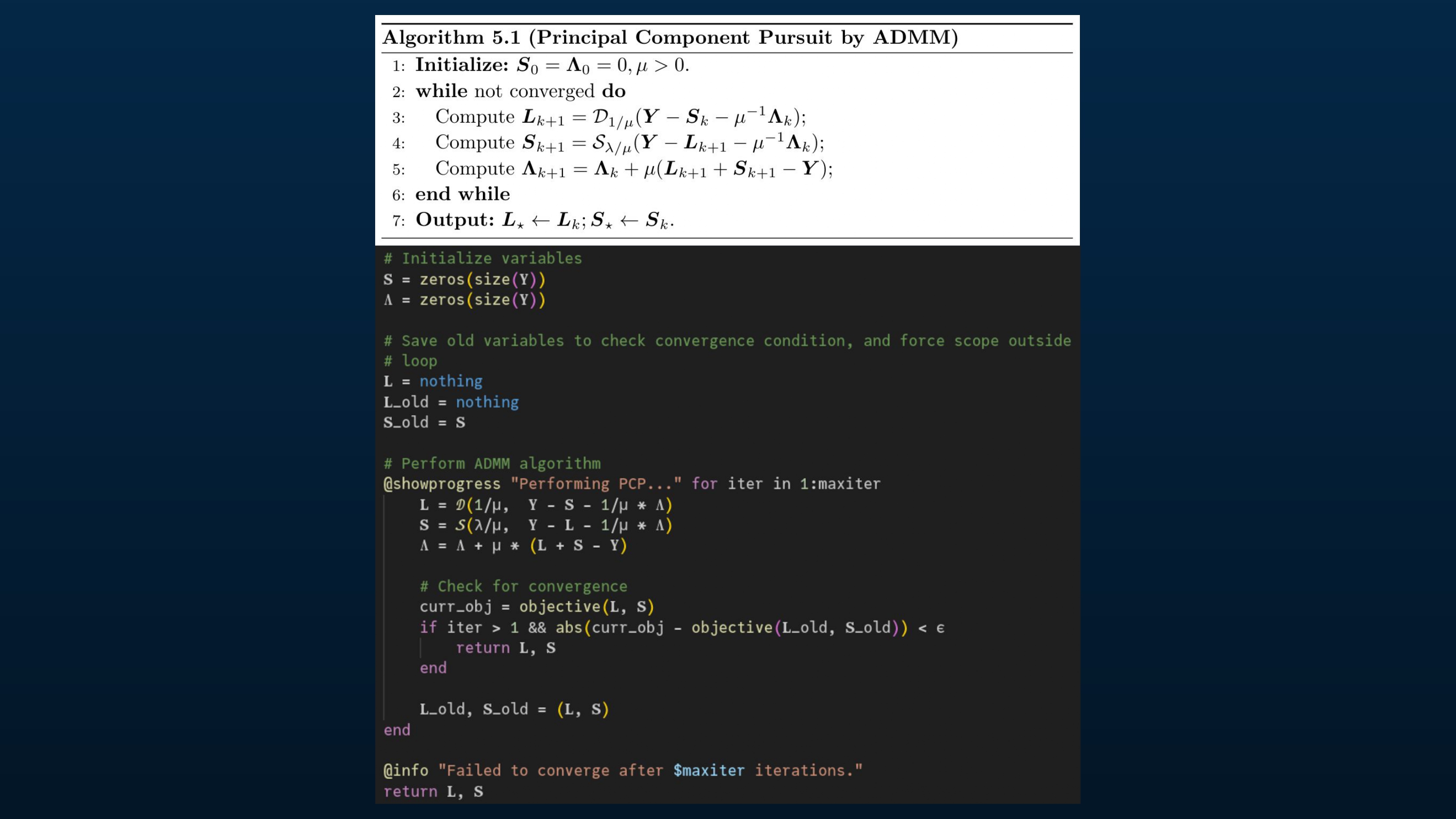
Wright and Ma provided pseudocode in their book for ADMM (Alternating Direction Method of Multipliers), an algorithm for solving convex optimization problems that happens to work well for this problem. I implemented it in Julia.

(I could have used a standard Julia library like Convex.jl, which would probably be more robust, but decided to implement the pseudocode to practice.)

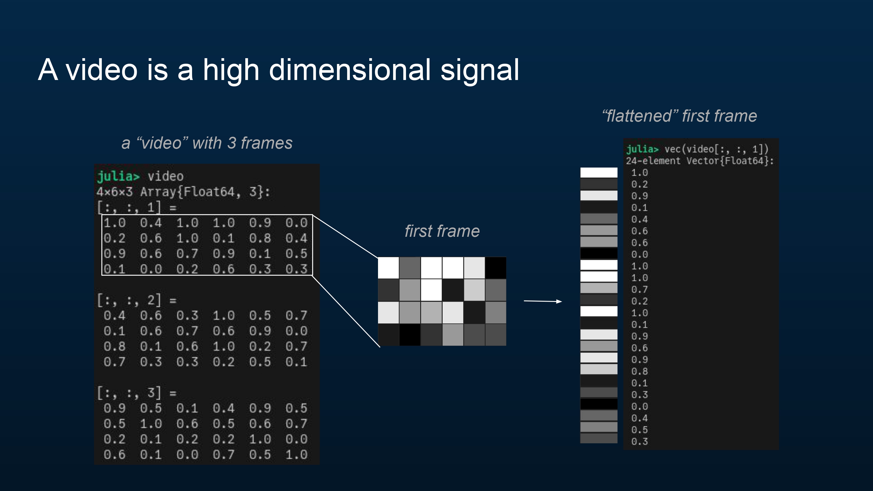
Now let’s talk about how a video fits into this whole framework, like the earlier video of me walking in my lab.

A video is a signal. For simplicity’s sake, I’m working with my videos in grayscale, but these methods should also apply (with some modifications) in color. Here I have an example “video” with three frames, each of which is just 4 by 6 pixels.

Each frame is a “block” of pixel intensity values. We can “flatten” each frame into a vector of values.

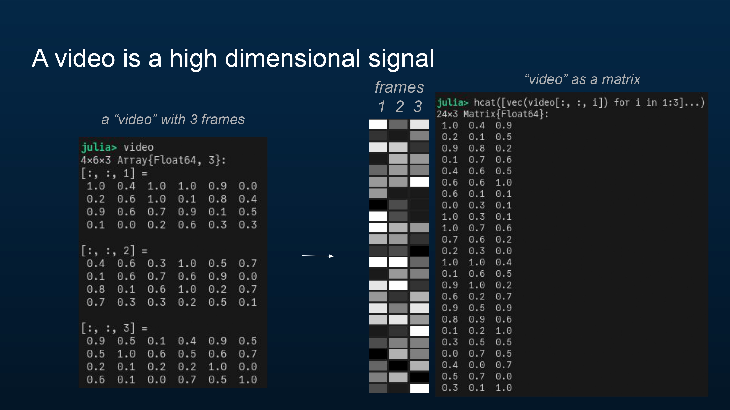
Applying this “flattening” to each frame of the video, we can convert the video (which is a 4×6×3 array) into a 24×3 matrix, where each column represents the signal at a point in time (a frame).

Now we’re ready to throw the video into the optimization problem previously described! I’ll set $\lambda = 1/\sqrt{\max(m, n)}$, where $\bold{Y}$ is $m \times n$, a rule-of-thumb suggestion by Wright and Ma in their book.

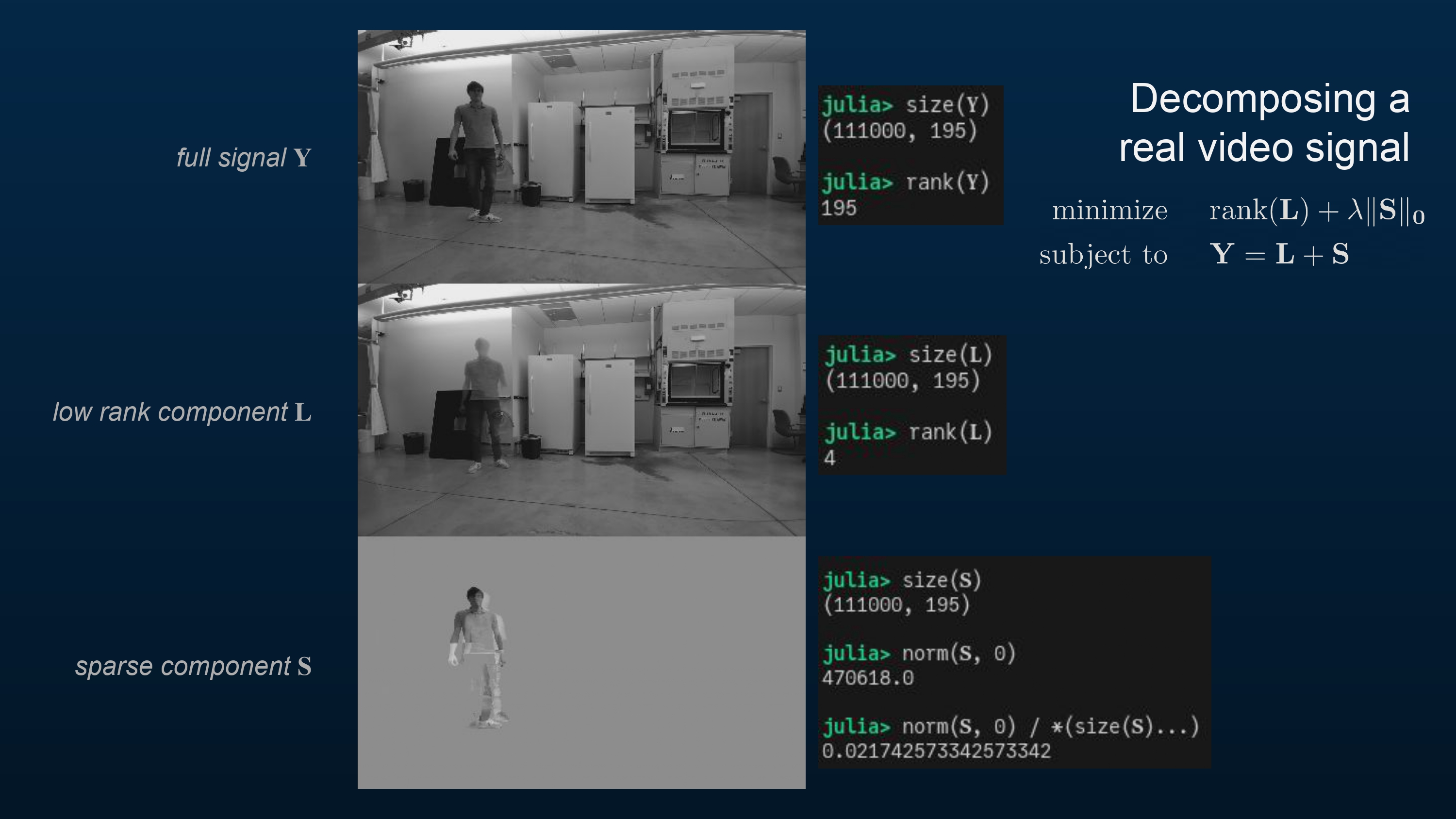
Here’s the video I showed earlier again. Each frame has 111,000 pixels, and there are 195 frames in the video, so $\bold{Y}$ is a 111,000×195 matrix. You can see that the rank of the original signal (the original grayscale video) is maximal, at 195.

After Principal Component Pursuit, the low-rank component has a rank of just 4. You can see that it only has a few unique frames—one where I’m standing with my hand seemingly chopped off (it was moving, so the algorithm added it to the sparse component), another where I’m not there at all, and another where I’m just visible by the fume hood.

The sparse component shows what was missing in the low-rank component, particularly, any part of the video that was moving. Only 2.2% of the pixels in the video are non-zero.

It looks like the new problem we constructed,

$$ \begin{aligned} \text{minimize}\quad&\Vert\bf{L}\Vert_* + \lambda \Vert\bf{S}\Vert_1 \\ \text{subject to}\quad&\bf{Y} = \bf{L} + \bf{S}, \end{aligned} $$

is a good replacement for the original problem

$$ \begin{aligned} \text{minimize}\quad&\text{rank}(\bf{L}) + \lambda \Vert\bf{S}\Vert_0 \\ \text{subject to}\quad&\bf{Y} = \bf{L} + \bf{S}! \end{aligned} $$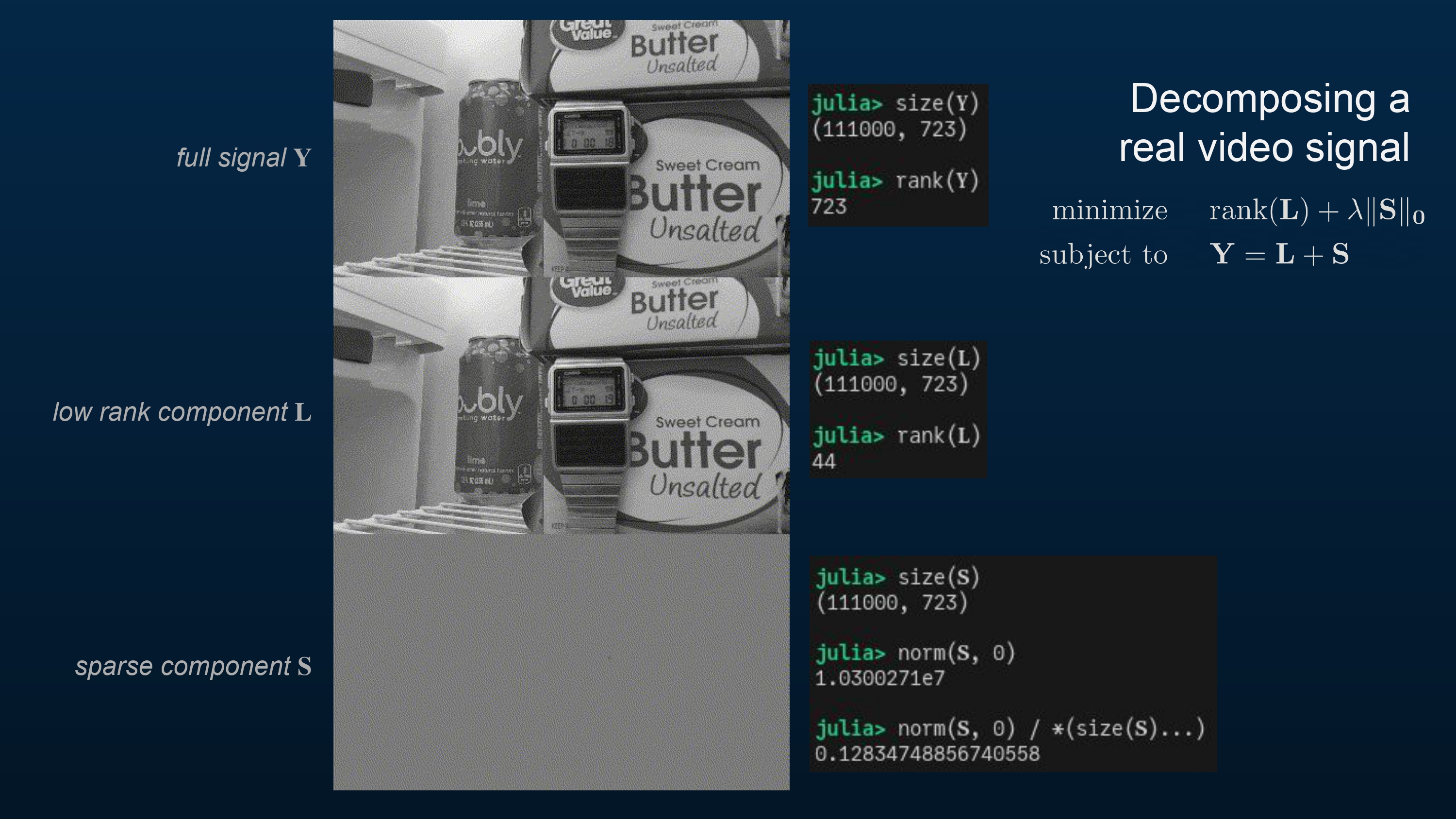

Here’s another demo.

The original video had 723 frames, and as before, 111,000 pixels per frame. Thus $\bold{Y}$ is a 111,000×723 matrix, with yet again full rank (723).

The low rank component isn’t as low rank as before, at 44. Perhaps a different choice of $\lambda$ would help here. Notice the digits displayed on the watch. It seems like 9 is Principal Component Pursuit’s favorite number!

About 12.8% of the pixels in the sparse component are non-zero.

Maybe this video is a little harder to decompose than the other one!

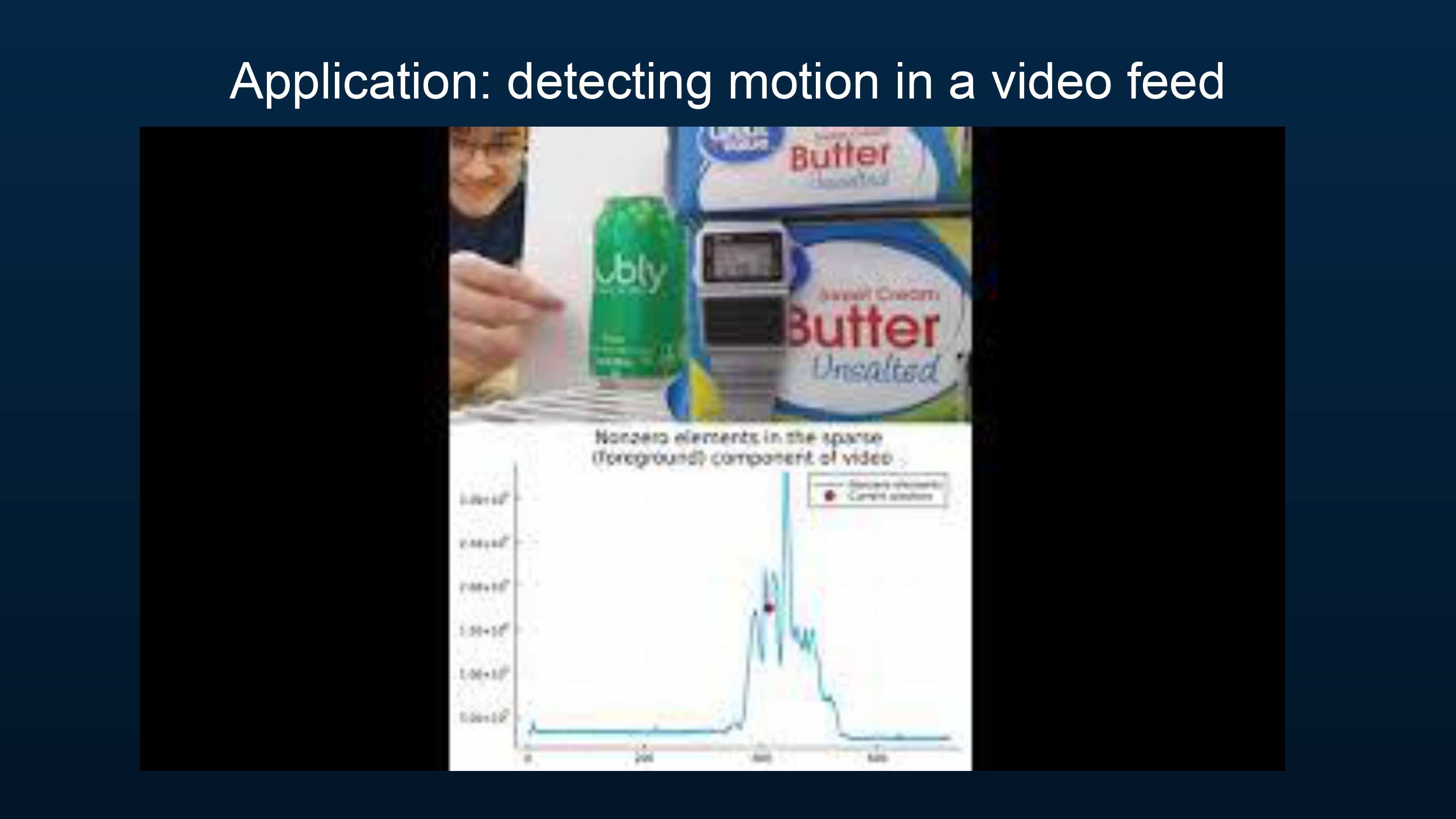
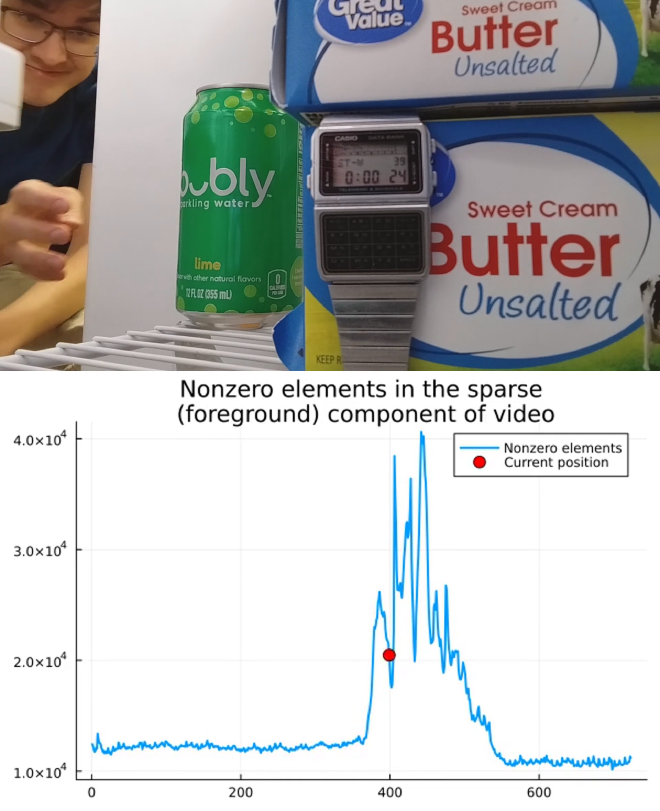
One simple application of this technique is to detect and quantify motion in a video. In this demo, I’ve counted the number of non-zero elements in each frame of the sparse component of the video and plotted it over time to measure motion.

(Here’s some bonus content—the same motion demo on the original video of me walking across the lab!)

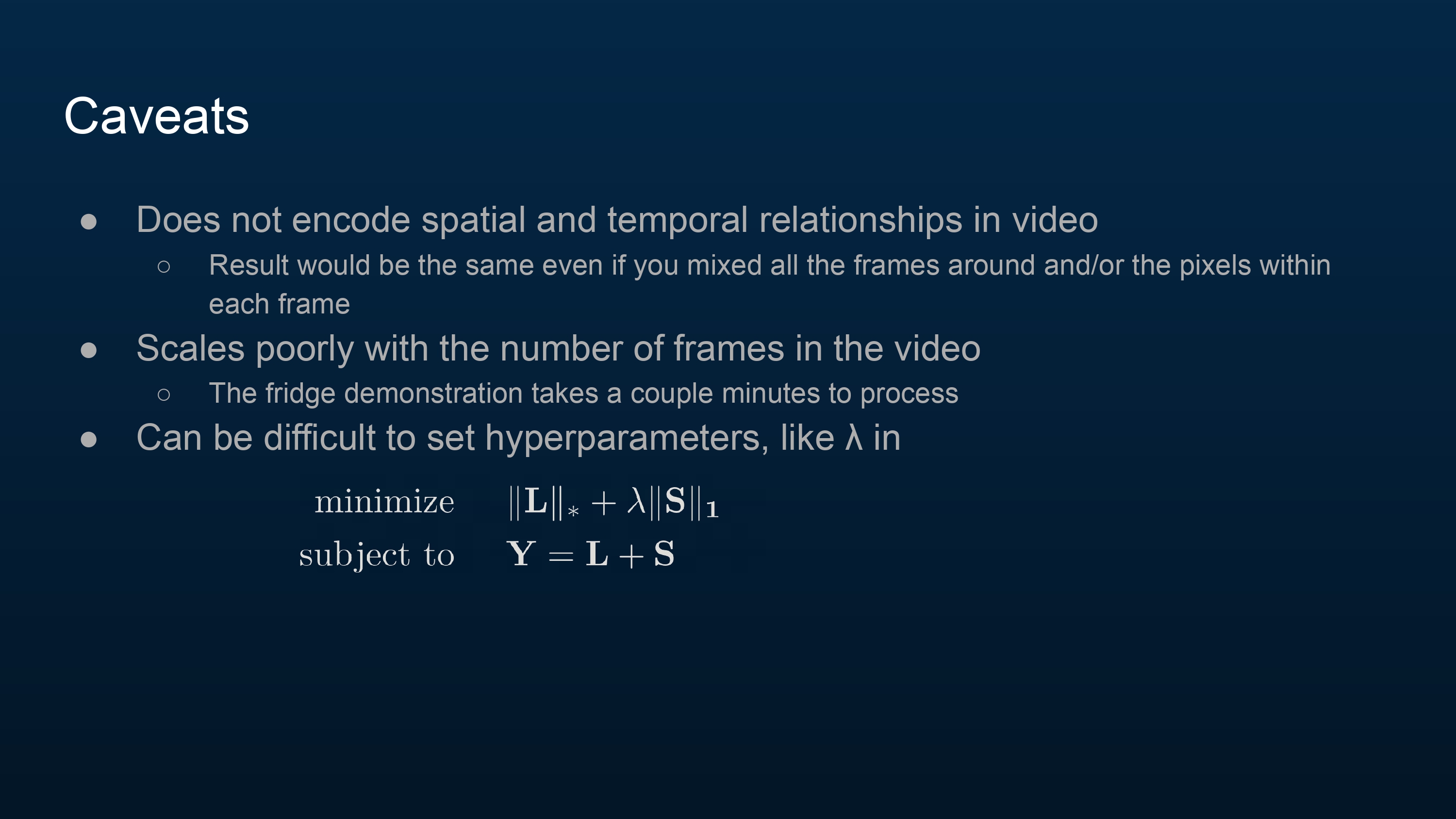
There are a number of issues with this approach.

It doesn’t take advantage of spatial and temporal relationships in video.
- We converted the video to a matrix $\bold{Y}$, where each column is a frame of the video, and each row is a single pixel’s intensity over time. Since all we’re concerning ourselves with is the rank and sparsity of the components of $\bold{Y}$, we could mix all the rows (frames) around and it wouldn’t make a difference (although it certainly should, especially in the context of the motion demo I did)! Likewise mixing the columns (pixels) around. No change.
It scales quite poorly with the length of the video.
- The walking-across-the-lab video took about 20 seconds on my ThinkPad to process, while the fridge video took a couple of minutes, even though the fridge video is only 3 or 4 times longer.
Setting $\lambda$ is difficult. A better choice of $\lambda$ might’ve helped in the fridge video demo.

References